In reinforcement learning (RL), an agent interacts with an environment over discrete time steps. At each step \(t\), the agent in state \(s_{t} \in S\) chooses an action \(a_{t} \in A\), receives a reward \(r_{t} = R(s_{t}, a_{t})\), and transitions to a new state \(s_{t+1}\) according to the probability \(P(s_{t+1} | s_{t}, a_{t})\). This setup is known as a Markov Decision Process (MDP), formally defined by the tuple \((S, A, P, R, \gamma)\), where \(S\) is the set of states, \(A\) is the set of actions, \(P\) is the transition probability, \(R\) is the reward function, and \(\gamma\) is the discount factor. The goal of RL is to learn a policy \( \pi_{\theta}(a\mid s) \), parameterized by \(\theta\), that maximizes the expected discounted return: $$ J(\theta) = \mathbb{E}_{\tau\sim\pi_{\theta}}\Bigl[\sum_{t=0}^{T-1}\gamma^{t}\,r_{t}\Bigr], $$ where a trajectory \(\tau = (s_{0},a_{0},r_{0},\dots)\) is generated by following \(\pi_{\theta}\). Training then amounts to solving the optimization $$ \theta^{*} \;=\; \arg\max_{\theta}\,J(\theta). $$ Let's make this more concrete with an example of a robot navigating a maze. The state might be the robot's current coordinates in the maze, and the action might be the direction it moves (e.g. up, down, left, right). Assign a reward of \(-1\) at each time step until the agent exits (to penalize long paths), and \(0\) upon reaching the goal. In this case, the optimal policy would be the one which minimizes the number of steps the robot takes to exit the maze. Now that we have an understanding of the RL problem, we can think about how to solve it. A natural way to approach the optimization problem is to use a gradient ascent strategy to iteratively improve the policy. This forms the core of policy gradient methods. In this blog, we will start with simple policy gradient methods such as REINFORCE, and work our way up to more sophisticated methods such as PPO.
REINFORCE
The REINFORCE algorithm is the simplest policy gradient method, which uses a Monte Carlo estimate of the gradient of the policy. To understand REINFORCE, we need to first compute the gradient of the objective function \(J(\theta)\) with respect to the policy parameters \(\theta\). We begin with the expected discounted return under policy \( \pi_\theta\): $$ J(\theta) = \mathbb{E}_{\tau\sim\pi_\theta}\Bigl[\sum_{t=0}^{T-1}\gamma^t\,r_t\Bigr] = \int P(\tau;\theta)\,R(\tau)\,d\tau, $$ where \(R(\tau)=\sum_{t=0}^{T-1}\gamma^t r_t\). Taking the gradient under the integral gives $$ \nabla_\theta J(\theta) = \int \nabla_\theta P(\tau;\theta)\,R(\tau)\,d\tau. $$ Applying the log-derivative trick \( \nabla_\theta P(\tau;\theta) = P(\tau;\theta)\,\nabla_\theta\log P(\tau;\theta) \) yields $$ \nabla_\theta J(\theta) = \int P(\tau;\theta)\,\nabla_\theta\log P(\tau;\theta)\,R(\tau)\,d\tau = \mathbb{E}_{\tau\sim\pi_\theta}\bigl[\nabla_\theta\log P(\tau;\theta)\,R(\tau)\bigr]. $$ Since $$ P(\tau;\theta) = P(s_0)\prod_{t=0}^{T-1}P(s_{t+1}\!\mid s_t,a_t)\,\pi_\theta(a_t\!\mid s_t), $$ we can write explicitly $$ \log P(\tau;\theta) = \log P(s_0) + \sum_{t=0}^{T-1}\Bigl[\log P(s_{t+1}\!\mid s_t,a_t) + \log \pi_\theta(a_t\!\mid s_t)\Bigr]. $$ Only the \( \log \pi_\theta \) term depends on \(\theta\), so $$ \nabla_\theta\log P(\tau;\theta) = \sum_{t=0}^{T-1}\nabla_\theta\log\pi_\theta(a_t\!\mid s_t). $$ Therefore the policy gradient becomes $$ \nabla_\theta J(\theta) = \mathbb{E}_{\tau\sim\pi_\theta}\Bigl[\sum_{t=0}^{T-1}\nabla_\theta\log\pi_\theta(a_t\!\mid s_t)\;R(\tau)\Bigr]. $$ Let's take a step back to think about what this gradient means. Intuitively, each action's log-probability gradient is weighted by its future reward, so good actions become more likely and bad actions less likely. In the case where each action's reward is the same, the gradient simplifies to the standard supervised learning gradient! Since the gradient is expressed in terms of an expectation, we can estimate it using a Monte Carlo sample by running our policy in the environment and computing the gradient of the log-probability of the actions taken. This gives the REINFORCE estimator: $$ \nabla_\theta J(\theta) \approx \frac{1}{N}\sum_{i=1}^N\sum_{t=0}^{T-1}\nabla_\theta\log\pi_\theta(a_t^{(i)}\!\mid s_t^{(i)})\;R(\tau^{(i)}). $$ This gives rise to the REINFORCE algorithm:
- Run the policy in the environment to collect a trajectory \(\tau^{(i)}\).
- Compute \(\nabla_\theta\log\pi_\theta(a_t^{(i)}\!\mid s_t^{(i)})\) and \(R(\tau^{(i)})\).
- Update the policy parameters \(\theta\) in the direction of the gradient. Specifically, $$ \theta \;\leftarrow\;\theta + \alpha \,\frac{1}{N} \sum_{i=1}^N\sum_{t=0}^{T-1}\nabla_\theta\log\pi_\theta(a_t^{(i)}\!\mid s_t^{(i)})\;R(\tau^{(i)}). $$
So far, I haven't stated anything about how the policy \(\pi_\theta\) is parameterized. This is a design choice, and there are many ways to parameterize a policy. For example, in the case of a robot navigating a maze with discrete actions, we could parameterize the policy as a MLP that takes in the state and outputs a softmax over the four actions. If we are in a continuous action space, we could parameterize the policy as a neural network that takes in the state and outputs the mean and standard deviation of a Gaussian policy. Then, we can sample an action from the policy by passing the state through the network and drawing a sample from the Gaussian. As long as the policy is differentiable, we can use the REINFORCE estimator to compute the gradient and update the policy parameters. Notice that we don't need to know anything about the state transition dynamics to compute the gradient!
High Variance in the Gradient Estimate
The REINFORCE algorithm can provide good results on simple tasks, but it suffers from high variance in the gradient estimate. This is because the gradient estimate is computed using a Monte Carlo estimate of the expected return, which can be quite noisy. A natural solution to this problem is to increase the number of samples used to estimate the gradient. While this will work, it greatly reduces the sample efficiency of the algorithm. In many environments, running the policy in the environment can be quite expensive. Let's take a look at the expression for the gradient estimate and see if we can come up with a better estimator. If we expand \(R(\tau^{(i)})\) in the expression for the gradient estimate, we get $$ \nabla_\theta J(\theta) \approx \frac{1}{N}\sum_{i=1}^N\sum_{t=0}^{T-1}\nabla_\theta\log\pi_\theta(a_t^{(i)}\!\mid s_t^{(i)})\;\Bigl[ \sum_{t'=0}^{T-1}\gamma^{t'}\,r_{t'}^{(i)} \Bigr]. $$ We can see that at timestep \(t\), the gradient estimate depends on the rewards at all timesteps \(t'\) in the trajectory. However, from our intuition on causality, the reward at timestep \(t\) should only depend on the actions taken after timestep \(t\). Here is a formal proof that we can sum the rewards only over the actions taken after timestep \(t\). This gives us the following estimator for the gradient: $$ \nabla_\theta J(\theta) \approx \frac{1}{N}\sum_{i=1}^N\sum_{t=0}^{T-1}\nabla_\theta\log\pi_\theta(a_t^{(i)}\!\mid s_t^{(i)})\;\Bigl[ \sum_{k=0}^{T-t-1}\gamma^{k}\,r_{t+k}^{(i)} \Bigr]. $$ The expression \(\sum_{k=0}^{T-t-1}\gamma^{k}\,r_{t+k}^{(i)}\) is commonly referred to as the reward-to-go. This estimator is still unbiased, but has lower variance since we have removed some of the noise in the gradient estimate.
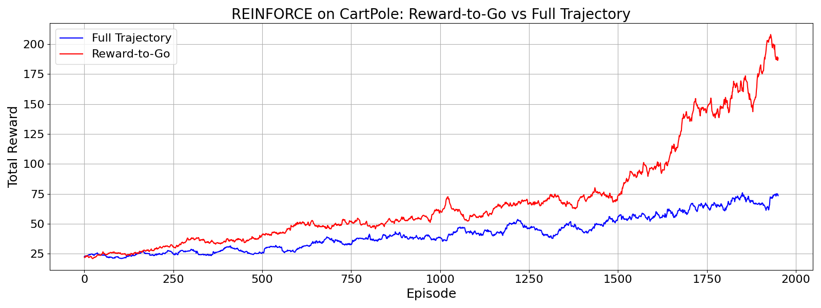
To make this more concrete, let's compare the performance of the REINFORCE algorithm with the reward-to-go estimator
compared to using the return from the full trajectory. I'll use the CartPole
environment from the OpenAI Gym. Below is a plot of the training performance of the REINFORCE algorithm with the reward-to-go estimator
A2C
Actor-Critic methods augment policy gradients with a learned value function to reduce variance. We maintain two parameterized functions:
- Policy (Actor): \(\pi_\theta(a\mid s)\), which outputs action probabilities (or parameters) given state \(s\).
- Value (Critic): \(V_\phi(s) = \mathbb{E}_{\tau\sim\pi_\theta}\bigl[\sum_{t=0}^\infty \gamma^t r_t \mid s_0 = s\bigr]\), the expected return from state \(s\).
Baselines
A key variance-reduction trick is to subtract a baseline \(b(s)\) from the return without biasing the gradient. Intuitively, if an action's return is exactly as expected (\(R = b\)), we don't update; if it's higher (lower), we upweight (downweight) the action. Without a baseline, if all the rewards are positive, the gradient will try to increase the probabilities of all actions seen in the trajectory. By adding a baseline, we help the gradient focus on upweighting the good actions and explicitly downweight the bad actions. Formally, for any function \(b(s)\): $$ \nabla_\theta J(\theta) = \mathbb{E}_{a\sim\pi_\theta}\bigl[\nabla_\theta \log \pi_\theta(a\mid s)\,(R - b(s))\bigr] $$ remains unbiased because $$ \mathbb{E}_{a\sim\pi_\theta}\bigl[\nabla_\theta \log \pi_\theta(a\mid s)\,b(s)\bigr] = b(s) \int \pi_\theta(a\mid s) \nabla_\theta \log \pi_\theta(a\mid s)\,da = b(s)\,\nabla_\theta \underbrace{\int \pi_\theta(a\mid s)\,da}_{=1} = 0. $$ Choosing \(b(s) = V_\phi(s)\) (the critic) yields the advantage: $$ A_t = Q_\phi(s_t,a_t) - V_\phi(s_t), $$ which centers the update and cuts variance.
n-Step Returns and Bias-Variance Tradeoff
To estimate \(Q\) and \(V\), we use n-step returns that interpolate between full Monte Carlo (high variance, low bias) and 1-step bootstrapping (low variance, higher bias). Define: $$ R_t^{(n)} = \sum_{k=0}^{n-1} \gamma^k\,r_{t+k} \;+\;\gamma^n\,V_\phi(s_{t+n}). $$
- When \(n\to\infty\), \(R_t^{(\infty)}\) is the full return (unbiased, but high variance).
- When \(n=1\), \(R_t^{(1)} = r_t + \gamma V_\phi(s_{t+1})\) (low variance, but biased by critic error).
- Intermediate \(n\) trades off bias (due to bootstrapping) vs. variance (due to sampling).
The advantage is then \(A_t = R_t^{(n)} - V_\phi(s_t)\). As \(n\) increases, variance grows but bias shrinks; in practice \(n\) is chosen (e.g., 5 or 20) to balance stable learning and sample efficiency.
A2C Algorithm:
- Collect \(n\)-step trajectories \(\{s_t,a_t,r_t\}\) (possibly across parallel actors).
- Compute for each \(t\):
- \(R_t^{(n)} = \sum_{k=0}^{n-1} \gamma^k\,r_{t+k} + \gamma^n V_\phi(s_{t+n})\).
- Advantage \(A_t = R_t^{(n)} - V_\phi(s_t)\).
- Actor update: \(\theta \gets \theta + \alpha_{\text{actor}}\,\mathbb{E}_t[\nabla_\theta \log \pi_\theta(a_t\mid s_t)\,A_t]\).
- Critic update: \(\phi \gets \phi - \alpha_{\text{critic}}\,\nabla_\phi\,\mathbb{E}_t\bigl(R_t^{(n)} - V_\phi(s_t)\bigr)^2\).
- Optional entropy bonus \(\beta\,\mathbb{E}_t[-\log\pi_\theta(a_t\mid s_t)]\) to encourage exploration.
- Repeat until convergence.
By combining a learned baseline and n-step bootstrapping, A2C achieves a lower-variance, more sample-efficient on-policy gradient than pure Monte Carlo methods.
TRPO
Trust Region Policy Optimization (TRPO) enforces a small “trust region” on each policy update to guarantee (under some assumptions) monotonic improvement of the expected return.
Rewriting the RL Objective
The exact change in return from \(\pi_{\rm old}\) to \(\pi_{\rm new}\) can be written as $$ J(\pi_{\rm new}) - J(\pi_{\rm old}) = \sum_{s} d^{\pi_{\rm new}}(s)\sum_{a}\pi_{\rm new}(a\!\mid\!s)\,A^{\pi_{\rm old}}(s,a), $$ where \(A^{\pi_{\rm old}}(s,a)=Q^{\pi_{\rm old}}(s,a)-V^{\pi_{\rm old}}(s)\) is the advantage under the old policy. Here \(d^{\pi}(s)\) is the discounted state-visitation frequency under policy \(\pi\). So, if the new policy has non-negative advantage in every state, then the new policy will have a higher return. What is particularly interesting is that the advantage is computed using the old policy. If you are familiar with policy iteration algorithms, then you might view policy gradient as a special case of policy iteration.
First-Order Surrogate via Taylor Expansion
It is not quite obvious how to optimize the above objective, since it requires knowing \(d^{\pi_{\rm new}}\) before updating, which means we need to sample from the new policy. It would be more desirable if we could use samples from the old policy to optimize the objective. Intuitively, this is a valid approximation when \(\pi_{\rm new}\) is close to \(\pi_{\rm old}\). Let \(L_{\pi_{\rm old}}(\pi) = J(\pi_{\rm old}) + \sum_{s}d^{\pi_{\rm old}}(s)\sum_{a}\pi(a\!\mid\!s)\,A^{\pi_{\rm old}}(s,a)\). Then \(L_{\pi_{\rm old}}(\pi)\) is a first-order approximation to \(J(\pi)\) around the old policy. Therefore, if we take small enough steps on the surrogate objective to make sure our local approximation is valid, we can guarantee monotonic improvement in the objective.
Forming a Trust Region
Let's think about how we can control the approximation error to make sure our local approximation is valid. Since we are making a first-order approximation of the objective, we are omitting higher-order information like curvature. In areas of large curvature, the first-order approximation can be quite inaccurate. In the case of RL policies, curvature is essentially the KL divergence between the old and new policies. Therefore, we can control the approximation error by ensuring that the KL divergence between the old and new policies is not too large. One can show that for some constant \(C\), $$ J(\pi_{\rm new}) \;\ge\; L_{\pi_{\rm old}}(\pi_{\rm new}) \;-\; C\,\bar D_{\mathrm{KL}}\bigl(\pi_{\rm old}\,\|\;\pi_{\rm new}\bigr), $$ where \(\bar D_{\mathrm{KL}}=\mathbb{E}_{s\sim d^{\pi_{\rm old}}}[D_{\mathrm{KL}}(\pi_{\rm old}(\cdot\!\mid\!s)\,\|\;\pi_{\rm new}(\cdot\!\mid\!s))]\).
Taking a step back, we have lower bounded the true RL objective by a surrogate objective with a KL divergence penalty. Since this surrogate objective is tangent to the true objective at the old policy, improving the KL penalized surrogate objective is guaranteed to improve the true objective. Therefore, we can maximize the KL penalized surrogate objective to improve the true objective. In practice, we solve the constrained optimization problem $$ \begin{aligned} &\max_{\pi}\;L_{\pi_{\rm old}}(\pi),\\ &\text{s.t.}\quad \bar D_{\mathrm{KL}}\bigl(\pi_{\rm old}\,\|\;\pi\bigr)\;\le\;\delta, \end{aligned} $$ where \(\delta\) is a small hyperparameter controlling the maximum average KL divergence per update.
Efficiently Solving the Constrained Optimization Problem
Calculating the KL divergence exactly is computationally expensive, since it requires computing \(\pi_\theta(a\mid s)\) for all \(s\) and \(a\). Instead, we can use a second-order approximation to the KL divergence that tends to work well in practice. $$ \bar D_{\mathrm{KL}}\bigl(\pi_{\rm old}\,\|\;\pi\bigr) \approx \tfrac12\,(\pi - \pi_{\rm old})^\top\,F\,(\pi - \pi_{\rm old}), $$ where \(F\) is the Fisher information matrix. The Fisher information matrix is just the Hessian of the KL divergence. You can work through the math yourself to see why the zeroth and first order terms vanish when approximating the KL divergence.
Putting it all together, our final optimization problem is $$ \begin{aligned} &\max_{\pi}\;L_{\pi_{\rm old}}(\pi),\\ &\text{s.t.}\quad \tfrac12\,(\pi - \pi_{\rm old})^\top\,F\,(\pi - \pi_{\rm old})\;\le\;\delta. \end{aligned} $$ This is a linear objective with a quadratic constraint. Let's take the Lagrangian of the optimization problem: $$ \mathcal{L}(\pi,\lambda) = L_{\pi_{\rm old}}(\pi) + \lambda\left(\tfrac12\,(\pi - \pi_{\rm old})^\top\,F\,(\pi - \pi_{\rm old}) - \delta\right). $$ Taking the gradient of the Lagrangian with respect to \(\pi\) and setting it to zero, we get $$ \nabla_\pi L_{\pi_{\rm old}}(\pi) + \lambda\,F\,(\pi - \pi_{\rm old}) = 0. $$ Solving for \(\lambda\), we get $$ \pi - \pi_{\rm old} = \frac{1}{\lambda}\,F^{-1}\,\nabla_\pi L_{\pi_{\rm old}}(\pi). $$ This is the natural gradient direction. So we can solve the optimization problem by backtracking along the natural gradient direction to enforce the KL constraint. It's worth noting that in practice, linear algebra tricks like conjugate gradient are used to avoid explicitly forming \(F^{-1}\).
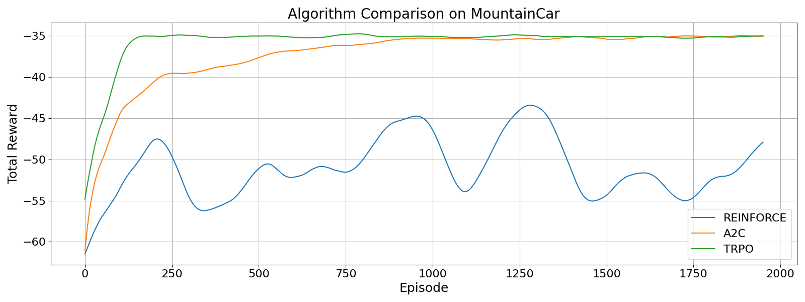
Below is the results of my implementation of TRPO on the MountainCar environment.
Since the reward signal is sparse, I used some reward shaping tricks for all the algorithms.
TRPO is able to learn faster than A2C and REINFORCE, but eventually my A2C implementation performs similarly.
Of course, there are many environments where TRPO far outperforms A2C - continuous control is a good example.
However, implenting all the tricks in TRPO is quite tricky and easy to get wrong.
This brings us to our next algorithm: Proximal Policy Optimization (PPO).
PPO
As we saw with TRPO, there is a lot of machinery and complexity needed to implement the algorithm. Additionally, TRPO requires second-order optimization methods to solve the problem. PPO aims to simplify the algorithm and rely on first-order optimization methods. To do this, PPO makes use of a clever clipping heuristic to prevent the policy from changing too much in each update, while still retaining the benefits of aggressive gradient steps.
Unpacking the PPO Objective
The core of PPO is the clipped surrogate objective: $$ L^{\mathrm{CLIP}}(\theta) = \mathbb{E}_t\Bigl[\min\bigl(r_t(\theta)\,A_t,\; \mathrm{clip}\bigl(r_t(\theta),\,1-\epsilon,\,1+\epsilon\bigr)\,A_t\bigr)\Bigr], $$ where $$ r_t(\theta) = \frac{\pi_\theta(a_t\mid s_t)}{\pi_{\theta_{\mathrm{old}}}(a_t\mid s_t)}, \quad A_t = R_t^{(n)} - V_\phi(s_t), $$ and \(\epsilon\) is a small constant (commonly \(0.1\) or \(0.2\)).
In practice, PPO augments the clipped policy loss with a value function loss and an entropy bonus to balance policy improvement, value accuracy, and exploration. The full PPO objective optimized per batch is: $$ L(\theta, \phi) = \mathbb{E}_t\Bigl[\,L^{\mathrm{CLIP}}(\theta) \;-\;c_1\,(V_\phi(s_t) - R_t^{(n)})^2 \;+\;c_2\,\mathcal{H}\bigl[\pi_\theta(\cdot\!\mid s_t)\bigr]\Bigr], $$ where:
- \(c_1\) weights the value function (critic) mean-squared error loss, ensuring the baseline stays accurate
- \(c_2\) weights the entropy bonus \(\mathcal{H}\), encouraging sufficient policy exploration
- \(R_t^{(n)} = \sum_{k=0}^{n-1} \gamma^k\,r_{t+k} + \gamma^n V_\phi(s_{t+n})\) is the n-step return
- \(V_\phi(s_t)\) is the critic's estimate of the state value
Here, \(r_t(\theta)\) measures how much the new policy's probability of the taken action has changed relative to the old policy. When \(r_t(\theta)\) stays within \([1-\epsilon,\,1+\epsilon]\), the first term \(r_t(\theta)\,A_t\) is used directly. This encourages actions that yielded positive advantage and discourages those with negative advantage. On the other hand, if the policy update it too large and \(r_t(\theta)\) is outside of the interval, the clipping operation caps it at the boundary. By clipping, we are zeroing out the gradient for the policy, which acts as a soft trust region. This prevents the policy update from acting greedily by creating large changes in the direction of positive reward, giving us the stability we want. Notice that by having the objective be the minimum of the unclipped and clipped objectives, PPO still penalizes large negative updates. So, we can view PPO as forming a pessimistic bound on the unclipped objective.
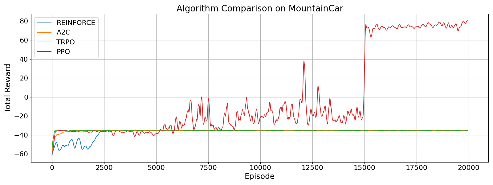
That's it! We have now seen the core of PPO. I implemented PPO on the MountainCar environment and compared it the TRPO, A2C, and REINFORCE algorithms.
The plot below shows that after enough training, PPO is able to reach far better performance than the other algorithms.
This showcases the simplicity and effectiveness of PPO and why it is now one of the most popular RL algorithms.
Conclusion
Policy gradient methods aim to use gradient ascent to improve the reinforcement learning objective. The simplest REINFORCE approach works well for simple tasks, but suffers from high variance in the gradient estimate. This motivated the development of Actor-Critic methods, which use a learned value function to reduce variance by computing advantage estimates. However, neither REINFORCE nor A2C consider the step size of the policy update. TRPO and PPO are two algorithms that address this issue by forming a trust region on the policy update. While inside this trust region, we can be confident that the linear approximation to the objective is reasonably accurate. TRPO takes a rigorous approach to forming this trust region by using the KL divergence between the old and new policies, while PPO uses a simpler clipping heuristic. In practice, PPO is simple to implement and achieves amazing results on complex tasks. This blog post did not cover a wide variety of other policy gradient methods, but I hope it gets across the core ideas.